Concept:
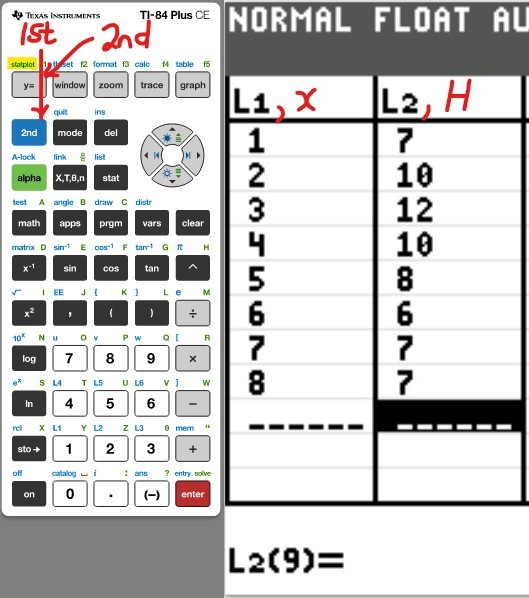
Table of Values
(a.) Given:
(i.) a polynomial
(ii.) several values of
x within constant increments
(b.) To Do:
(i) Determine values of
y
(ii) Make a Table of Values for the polynomial
(4.) In Calculus, certain functions can be approximated by polynomial
functions.
Explore such function now.
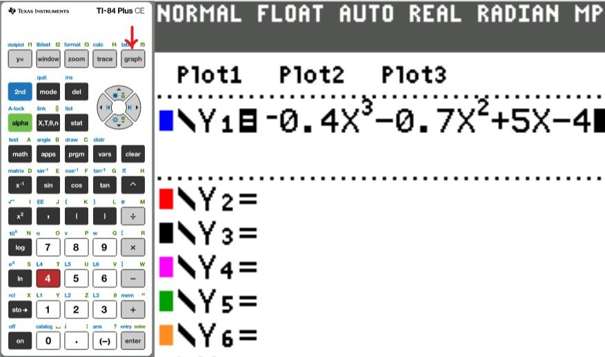
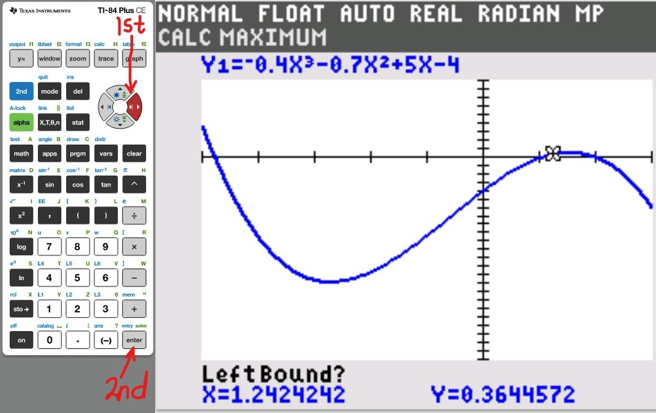
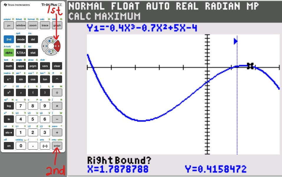
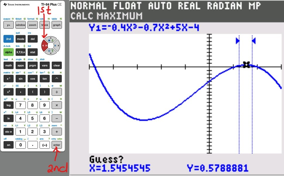
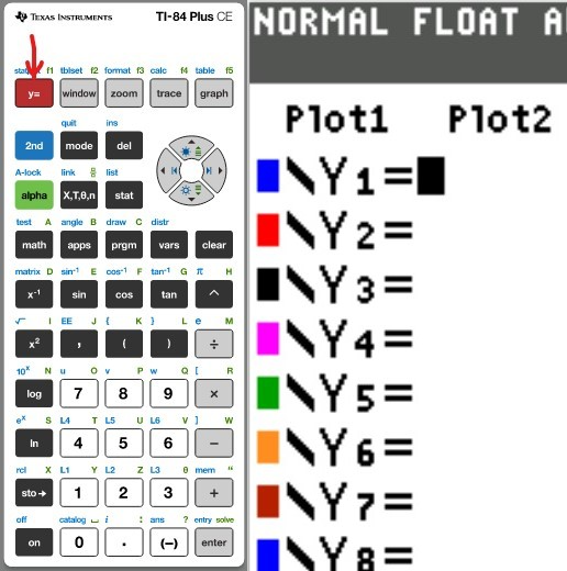
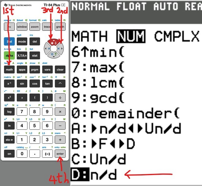
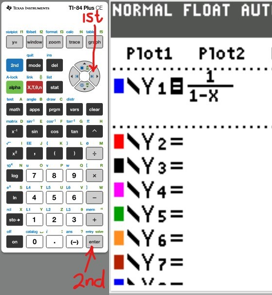
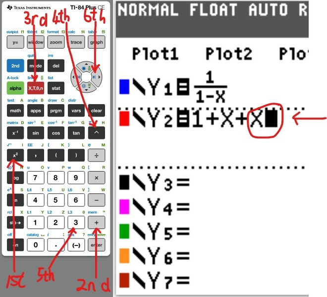
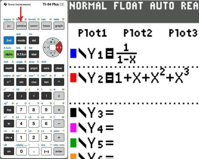
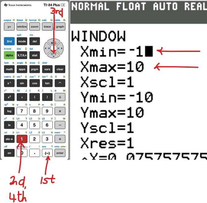
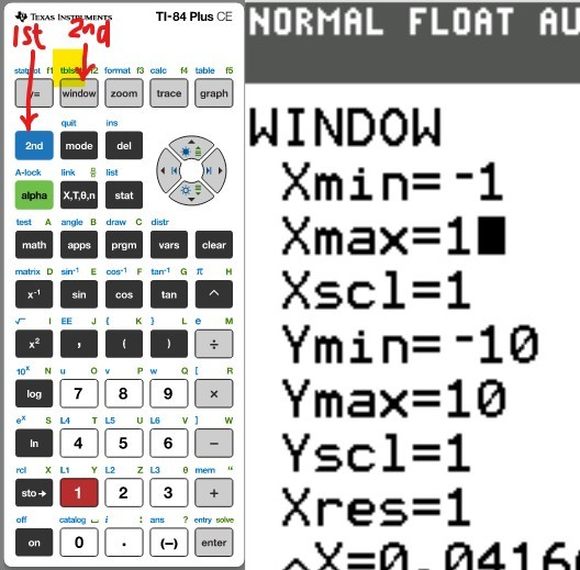
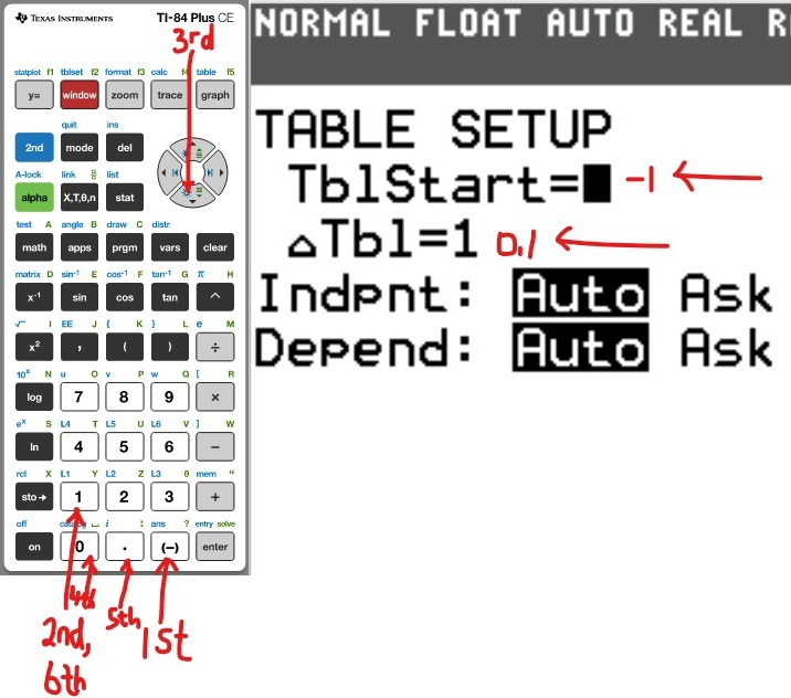
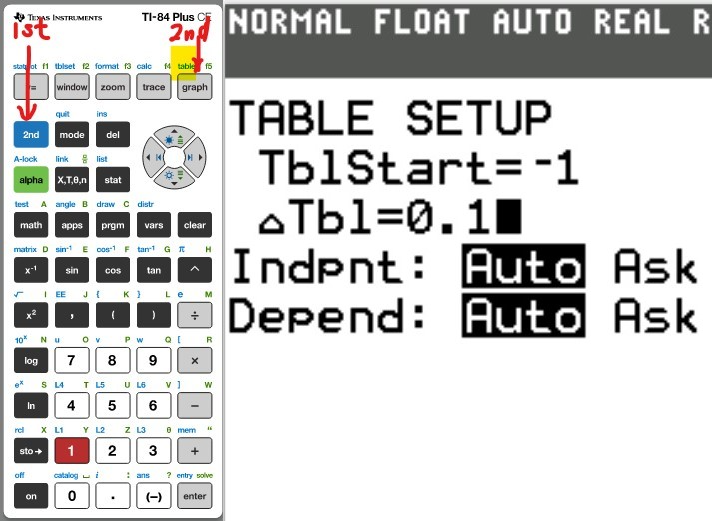
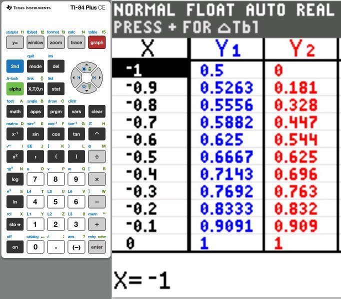
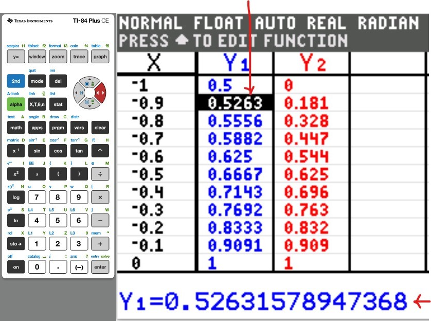
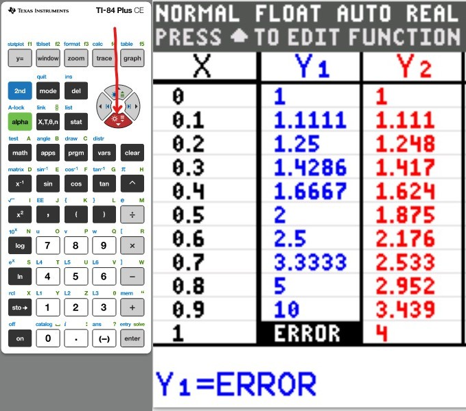
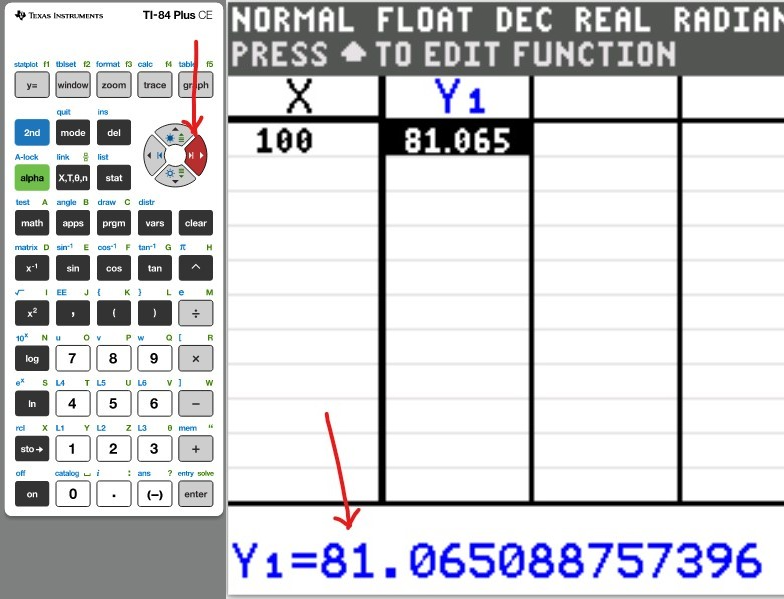
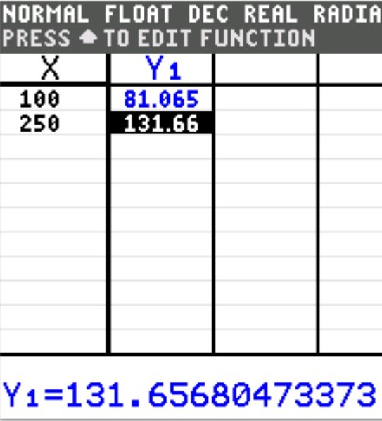
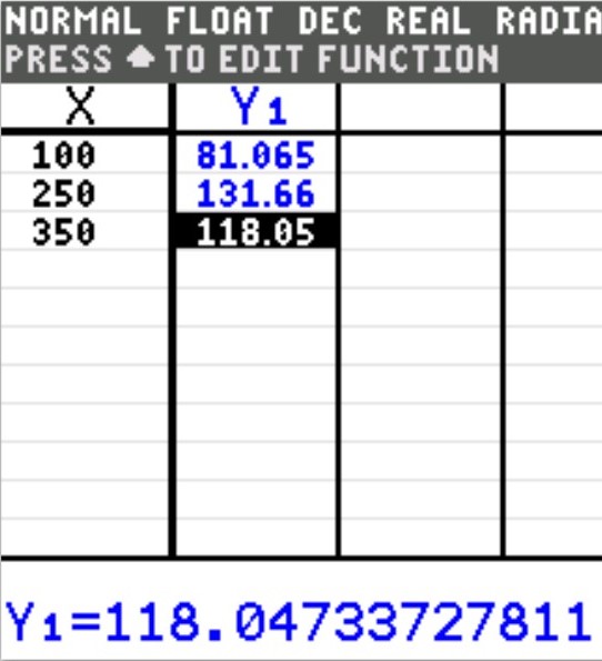
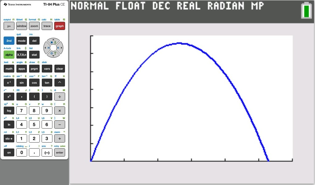
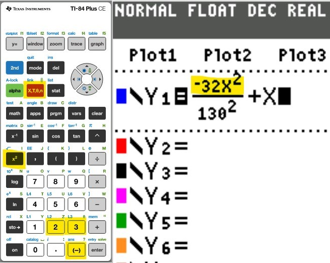
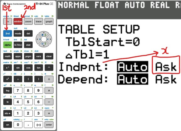
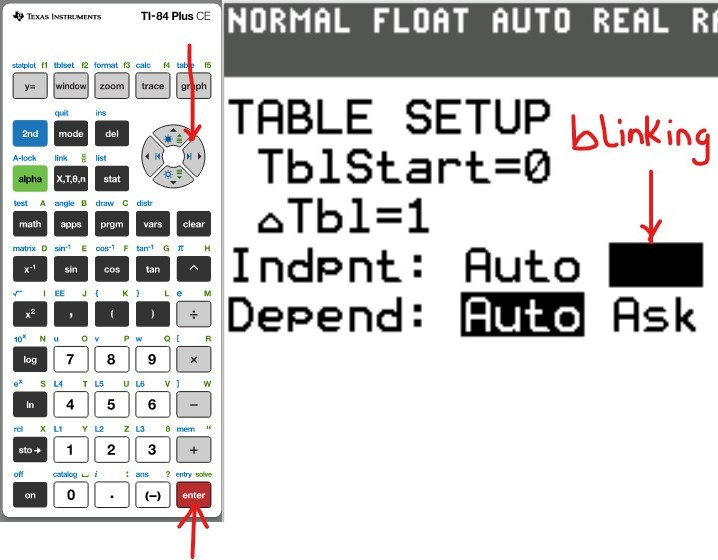
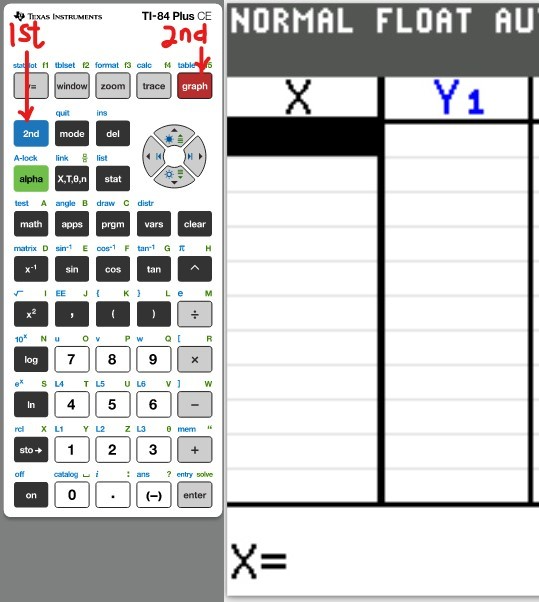
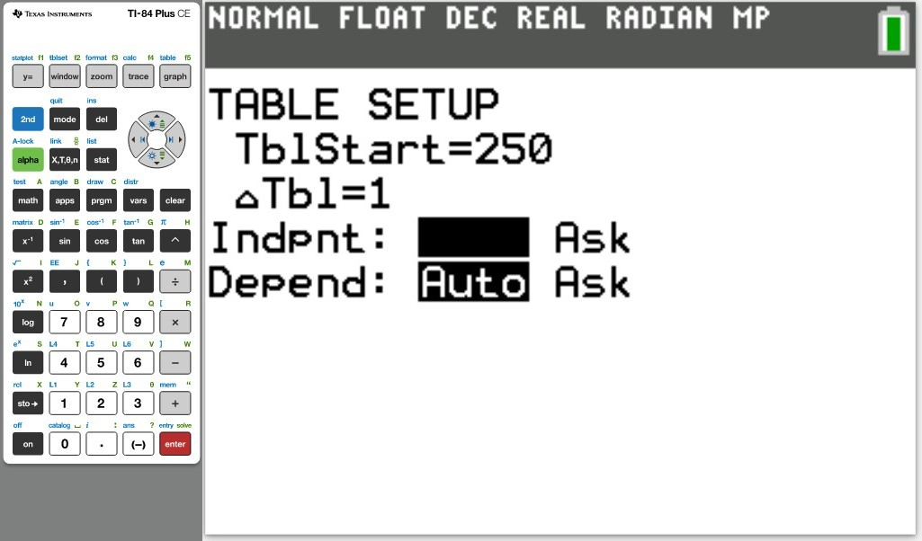
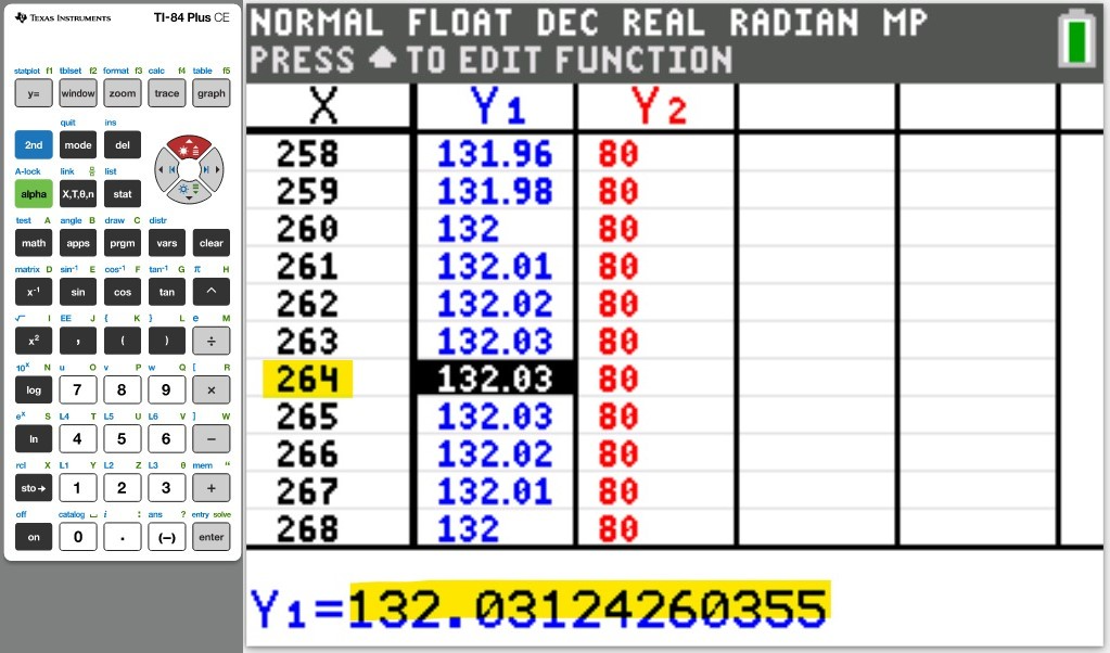
(a.) Using a graphing utility, create a table of values with $Y_1 = f_1(x) = \dfrac{1}{1 - x}$ and $Y_2 = g_1(x) = 1 + x + x^2 + x^3$ for $-1 \le x \le 1$ with $\Delta Tbl = 0.1$
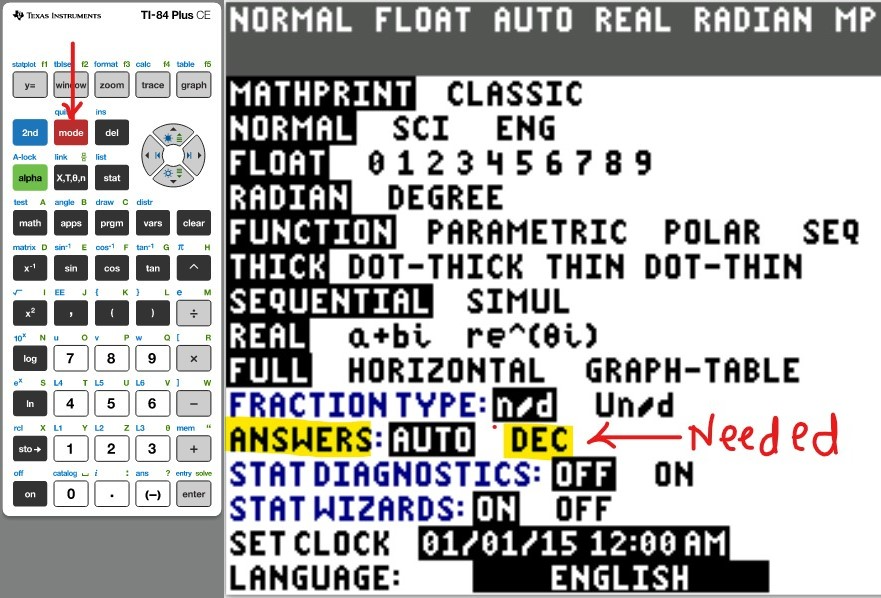
(Type an integer or decimal rounded to five decimal places as needed. Type N if the function is undefined).
| $x$ |
$Y_1$ |
$Y_2$ |
| −1 |
............ |
............ |
| −0.9 |
............ |
............ |
| −0.8 |
............ |
............ |
| −0.7 |
............ |
............ |
| −0.6 |
............ |
............ |
| −0.5 |
............ |
............ |
| −0.4 |
............ |
............ |
| −0.3 |
............ |
............ |
| −0.2 |
............ |
............ |
| −0.1 |
............ |
............ |
| 0 |
............ |
............ |
| 0.1 |
............ |
............ |
| 0.2 |
............ |
............ |
| 0.3 |
............ |
............ |
| 0.4 |
............ |
............ |
| 0.5 |
............ |
............ |
| 0.6 |
............ |
............ |
| 0.7 |
............ |
............ |
| 0.8 |
............ |
............ |
| 0.9 |
............ |
............ |
| 1 |
............ |
............ |
(b.) Using a graphing utility, create a table of values with $Y_1 = f_2(x) = \dfrac{1}{1 - x}$ and $Y_2 = g_2(x) = 1 + x + x^2 + x^3 + x^4$ for $-1 \le x \le 1$ with $\Delta Tbl = 0.1$
(Type an integer or decimal rounded to five decimal places as needed. Type N if the function is undefined).
| $x$ |
$Y_1$ |
$Y_2$ |
| −1 |
............ |
............ |
| −0.9 |
............ |
............ |
| −0.8 |
............ |
............ |
| −0.7 |
............ |
............ |
| −0.6 |
............ |
............ |
| −0.5 |
............ |
............ |
| −0.4 |
............ |
............ |
| −0.3 |
............ |
............ |
| −0.2 |
............ |
............ |
| −0.1 |
............ |
............ |
| 0 |
............ |
............ |
| 0.1 |
............ |
............ |
| 0.2 |
............ |
............ |
| 0.3 |
............ |
............ |
| 0.4 |
............ |
............ |
| 0.5 |
............ |
............ |
| 0.6 |
............ |
............ |
| 0.7 |
............ |
............ |
| 0.8 |
............ |
............ |
| 0.9 |
............ |
............ |
| 1 |
............ |
............ |
(c.) Using a graphing utility, create a table of values with $Y_1 = f_3(x) = \dfrac{1}{1 - x}$ and $Y_2 = g_3(x) = 1 + x + x^2 + x^3 + x^4 + x^5$ for $-1 \le x \le 1$ with $\Delta Tbl = 0.1$
(Type an integer or decimal rounded to five decimal places as needed. Type N if the function is undefined).
| $x$ |
$Y_1$ |
$Y_2$ |
| −1 |
............ |
............ |
| −0.9 |
............ |
............ |
| −0.8 |
............ |
............ |
| −0.7 |
............ |
............ |
| −0.6 |
............ |
............ |
| −0.5 |
............ |
............ |
| −0.4 |
............ |
............ |
| −0.3 |
............ |
............ |
| −0.2 |
............ |
............ |
| −0.1 |
............ |
............ |
| 0 |
............ |
............ |
| 0.1 |
............ |
............ |
| 0.2 |
............ |
............ |
| 0.3 |
............ |
............ |
| 0.4 |
............ |
............ |
| 0.5 |
............ |
............ |
| 0.6 |
............ |
............ |
| 0.7 |
............ |
............ |
| 0.8 |
............ |
............ |
| 0.9 |
............ |
............ |
| 1 |
............ |
............ |
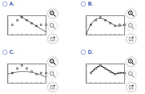
(d.) What do you notice about the values of the function as more terms are added to the polynomial?
Are there some values of
x for which the approximations are better?
A. As more terms are added, the values of the polynomial function get further and further away from the values of
f.
The approximations near −1 or 1 are better than those near 0.
B. As more terms are added, the values of the polynomial function get closer to the values of
f.
The approximations near 0 are better than those near −1 or 1.
C. As more terms are added, the values of the polynomial function get further and further away from the values of
f.
The approximations near 0 are better than those near −1 or 1.
D. As more terms are added, the values of the polynomial function get closer to the values of
f.
The approximations near −1 or 1 are better than those near 0.
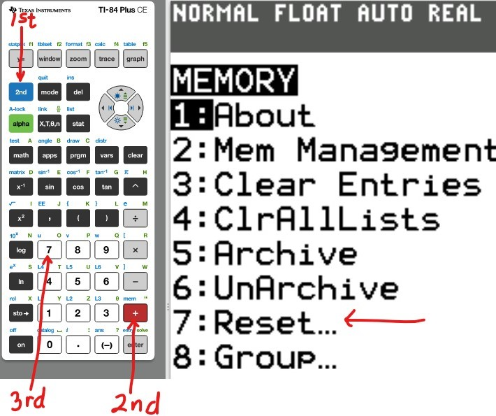
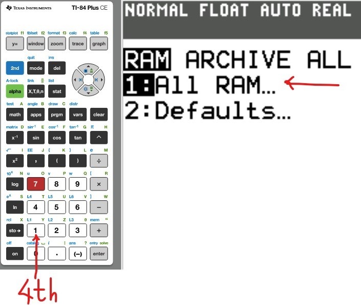
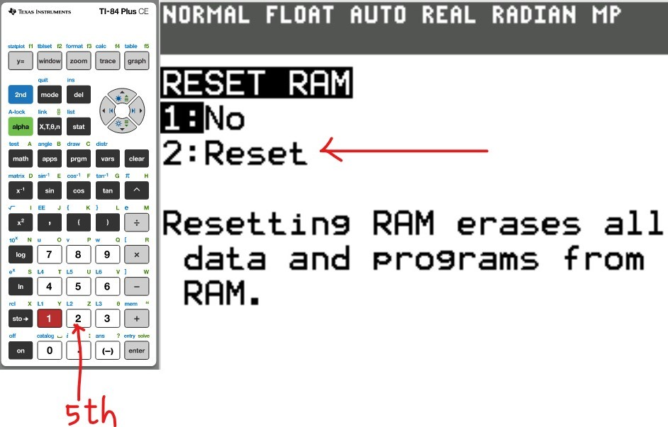
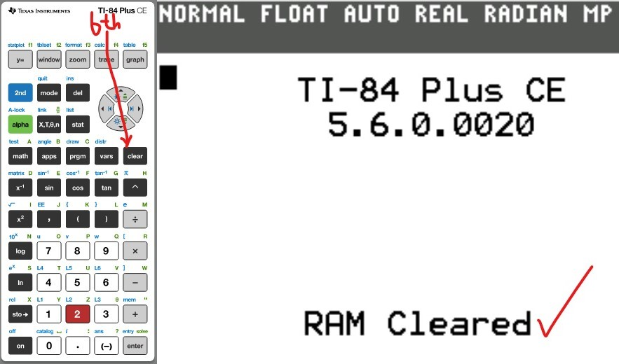
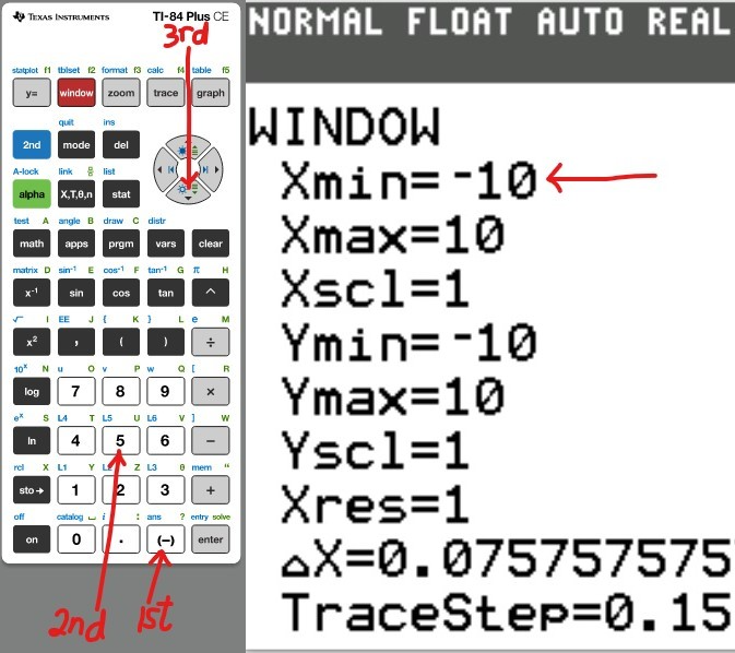
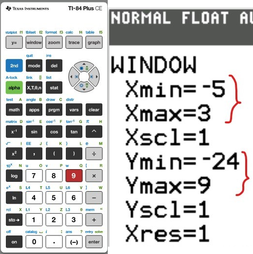
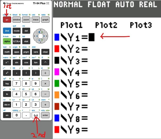
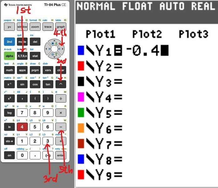
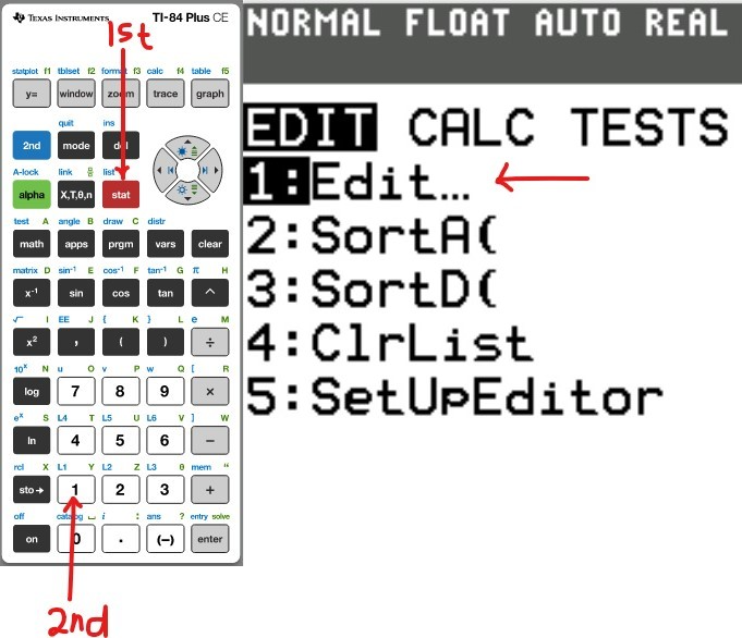
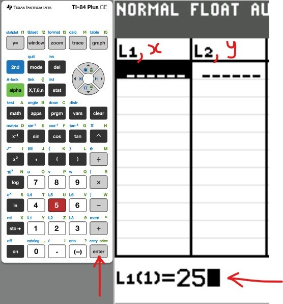
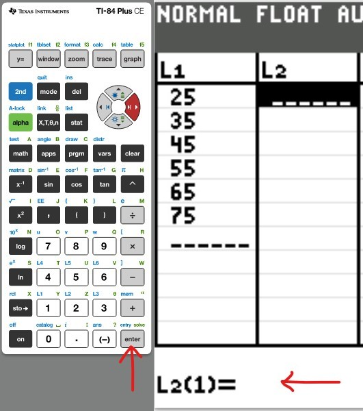
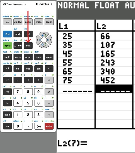
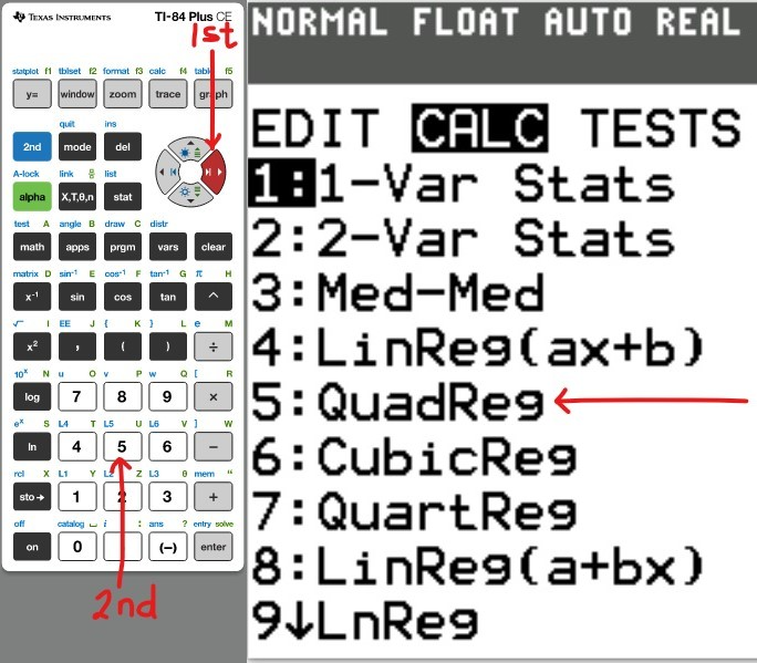
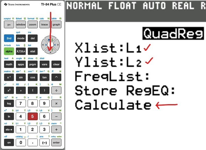
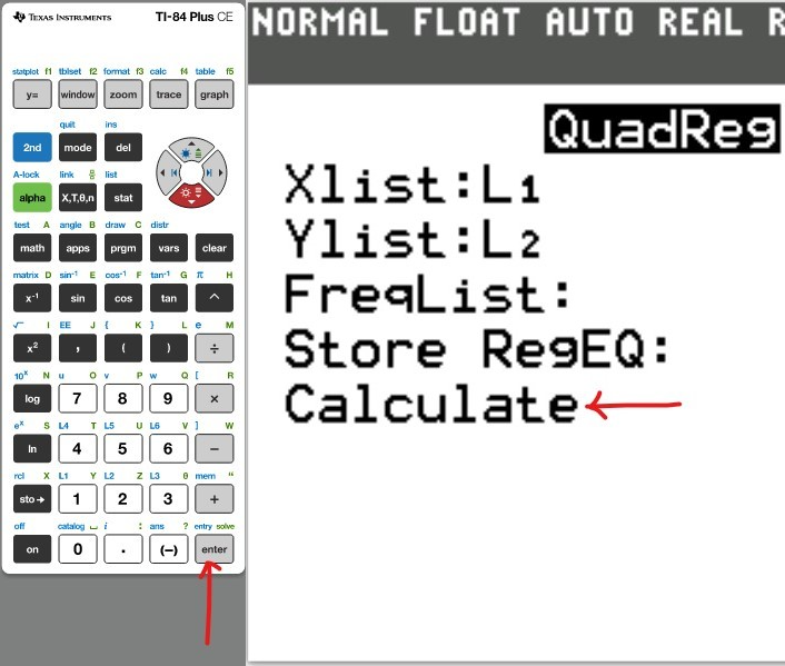
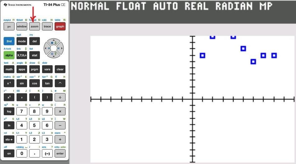
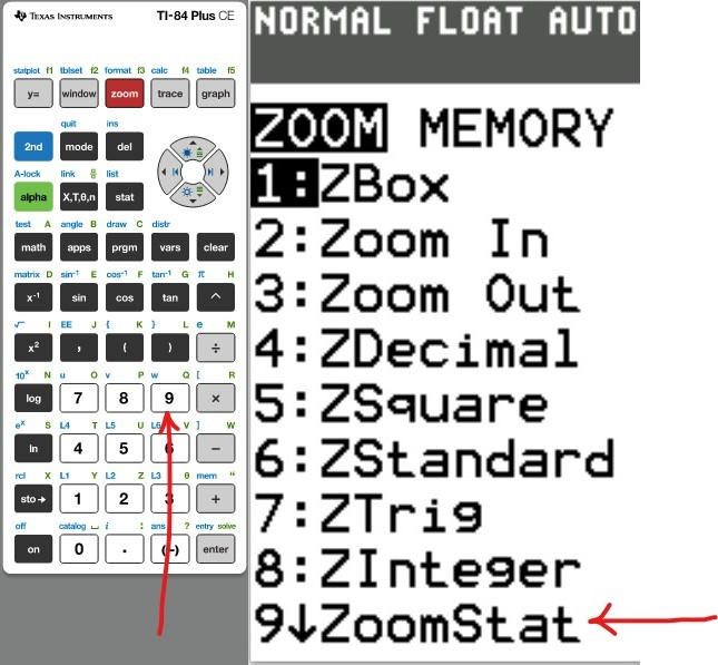
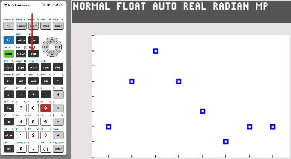
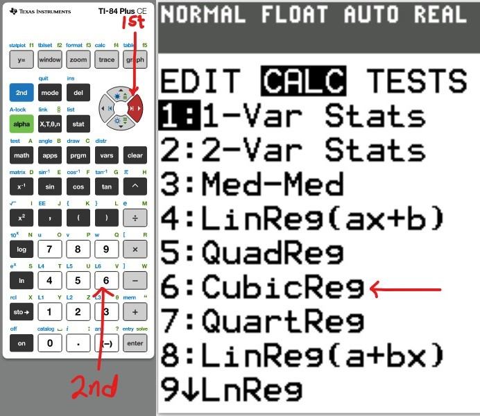
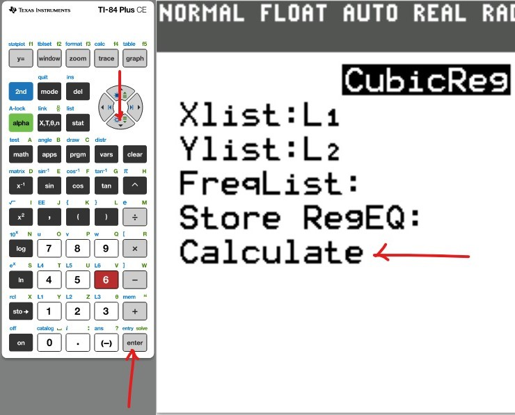
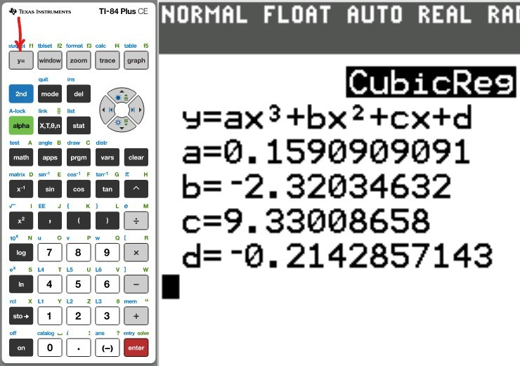
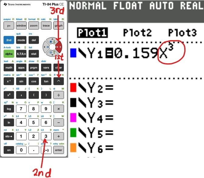
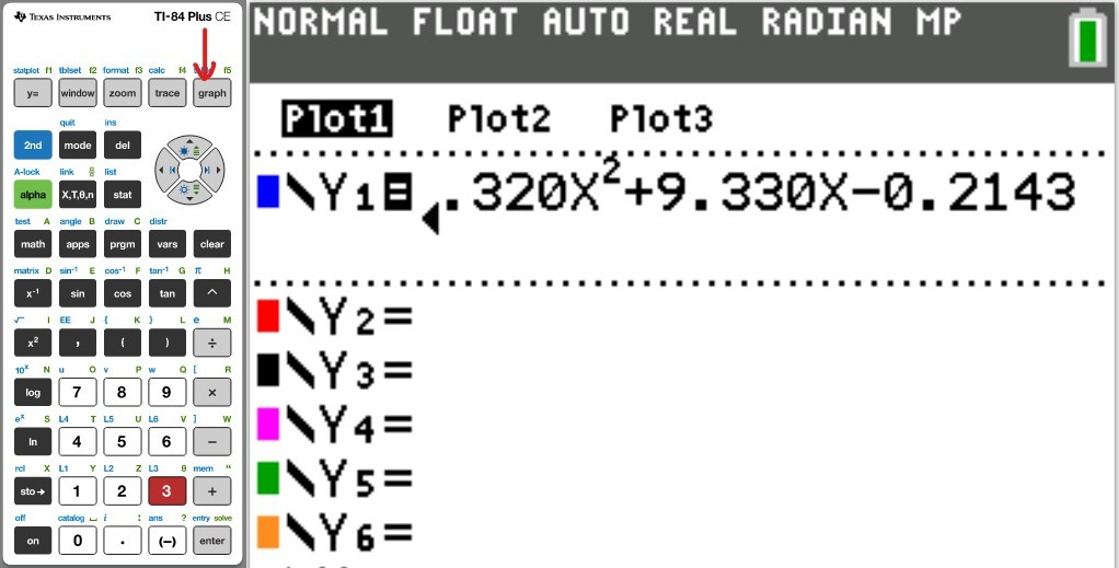
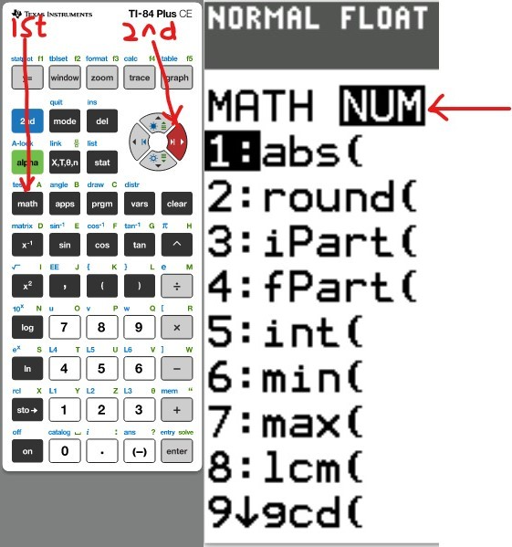
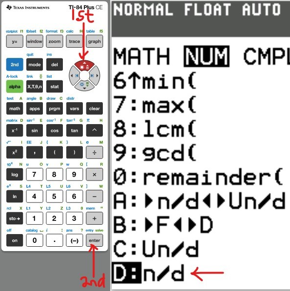
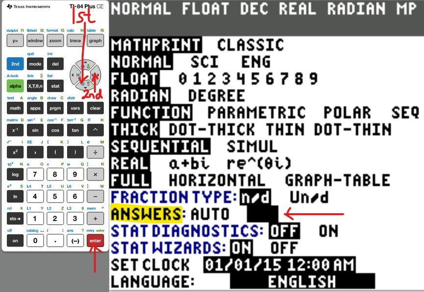
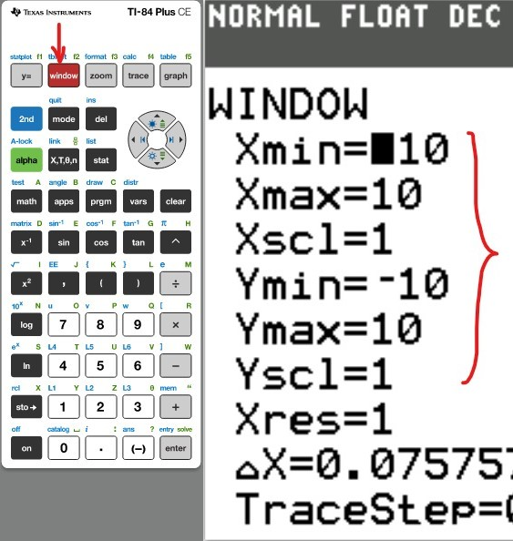
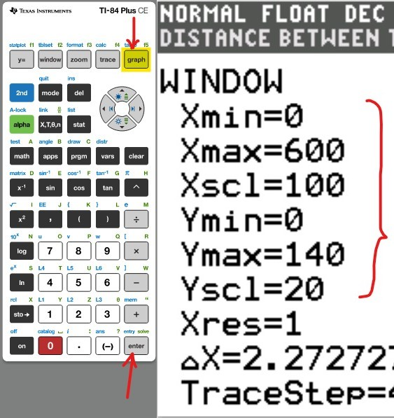
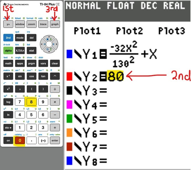
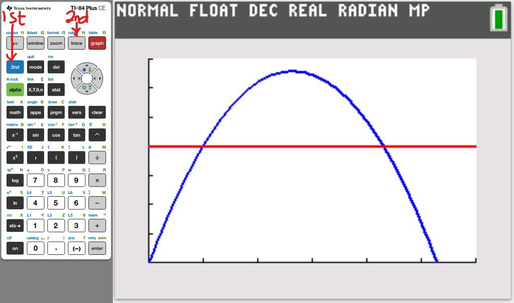
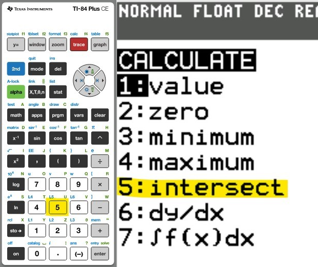
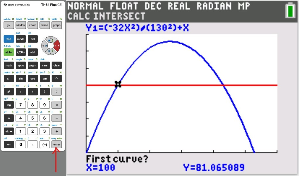
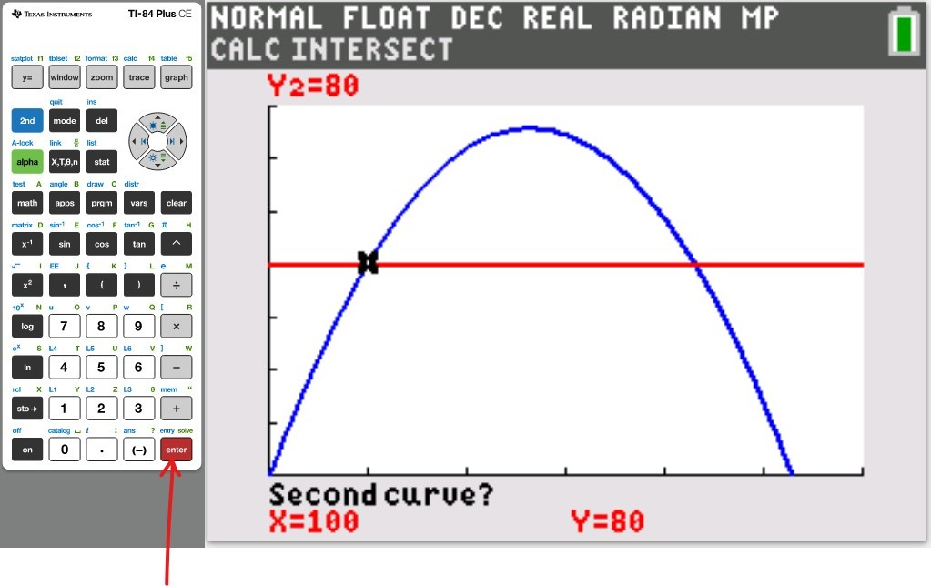
 You may use any of these TI calculators: